Methods for Automated Change Detection using Remote Sensing Data
Michael Evans, Defenders of Wildlife
2017-12-12
Summary
The Center for Conservation Innovation at Defenders of Wildlife has been developing methods to use the increasing abundance of remote sensing data to inform and improve imperiled species conservation. Our goal is to develop a set of generalized methods that can be applied in a variety of landscapes to detect land cover changes. We have used these methods to detect habitat disturbance from energy development and agricultural conversion across the range of the lesser prairie chicken, and are currently tracking the appearance and growth of sand mining in the range of the dunes sagebrush lizard in west Texas. There are many ways to use these analytical tools for conservation, and we will continue to develop and use them in other contexts, both independently and in collaboration with conservation partners.
Remote Sensing
In this document, the term ‘remote sensing’ describes the measurement of electromagnetic reflectance (e.g., visible, ultraviolet, and infrared light waves) from the Earth’s surface by sensors on satellites or airplanes. These values are stored as images, and are used to quantify patterns of land cover and land use. A recent proliferation of such data has increased the use of remote sensing in conservation. Many satellite systems collect new images across the globe bi-weekly, advancing the ability to quickly detect and quantify habitat loss. Below are common terms used in discussions of remote sensing:
Pixel: a (usually square) data point in an image storing the reflectance and other data values at a given location. Pixels may contain values for multiple different variables and data types.
Band: a single variable recorded at pixels in an image. Images may contain many bands at each pixel, often storing values from different parts of the electromagnetic spectrum. However, bands can also contain supplementary information at each pixel such as elevation, date of collection, or derived variables.
Resolution: the size of an image’s pixels, usually as measured by one side of the pixel (e.g., 10m, or 1km resolution). Equivalently, the number of pixels per unit area. Higher resolution (i.e. smaller pixels) images provide more detail by capturing fine scale variation in reflectance across a given area.
Historically, satellites collected more frequent data while photos taken from airplanes (i.e. aerial photos), provided higher resolution. However, as costs have decreased, more and more satellite systems are being deployed collecting high resolution (<3m) data at frequent intervals (<5d). Thus far, our work has primarily used three data sources:
Landsat-8 is a satellite system deployed and maintained by the U.S. Geological Survey, providing global coverage of 30-meter resolution imagery every 16 days. Landsat-8 images contain 12 bands that record reflectance values in the visible (RGB), near infrared, short-wave infrared and near ultraviolet spectra. 1
Sentinel-2 is a satellite system deployed and maintained by the European Space Agency, providing global coverage of 10-meter resolution imagery every 12 days. Sentinel-2 images contain 12 bands that record reflectance values in the visible, near infrared, short-wave infrared and near ultraviolet spectra. 2
The National Agricultural Imagery Program (NAIP) is run by the U.S. Department of Agriculture, and acquires 1-meter resolution aerial imagery during the agricultural growing seasons in the continental U.S. NAIP imagery usually contains 4 bands recording reflectance in the visible and near infrared spectra. Images are collected annually per state, and national coverage occurs in 3 year cycles3.
Automated Change Detection
Automated change detection describes the process of using algorithms and/or machine learning to identify areas at which land cover changes between two time points. For detecting changes across large areas, or with high frequency, automation can improve speed and reliability over manually examining before and after images for change. We use Google Earth Engine — a platform providing real-time access to terabytes of remote sensing data and the cloud computing capabilities to analyze them — to create a process to automatically detect changes in land use and land cover between two time periods. The basic process involves the following key steps:
- Acquire satellite data from before and after the date of interest.
- Calculate changes in the Earth’s surface reflectance values using the data.
- Identify minimum changes in reflectance values that correspond to the habitat loss we want to identify.
- Select pixels exceeding these minimum changes.
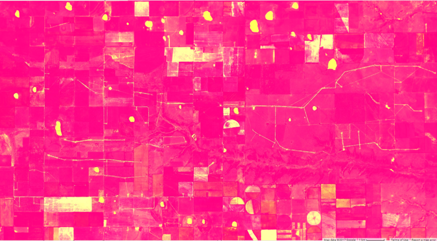
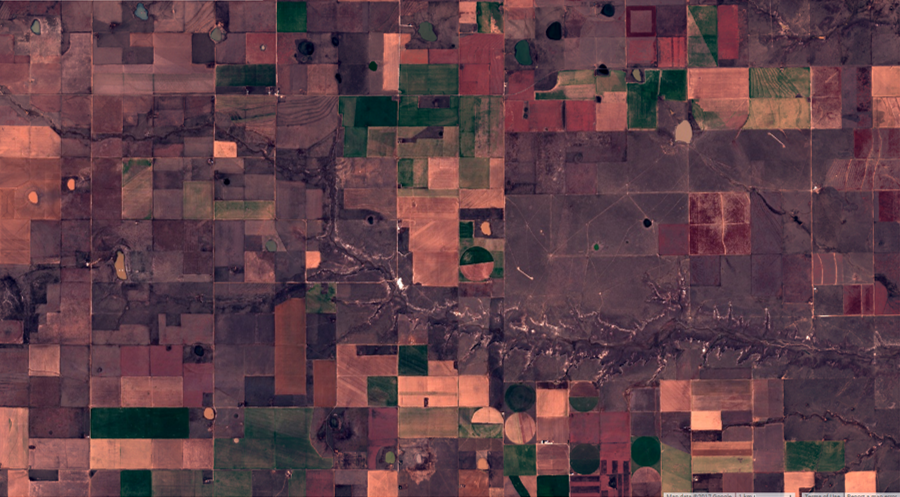

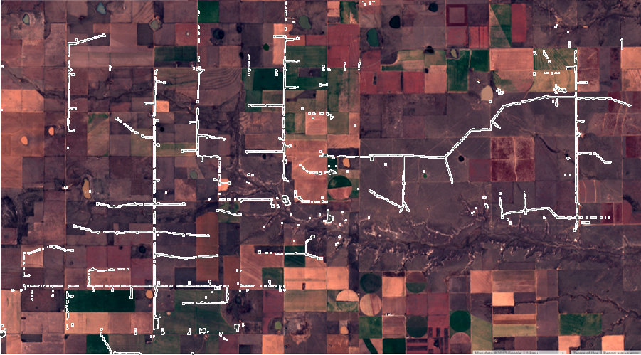
Figure 1. The process of automated land cover change detection, illustrated with images at a Texas wind farm constructed after September 2015. Use the sliders to see the raw changes in reflectance values calculated between September 1, 2015 an April 1, 2017 (top) and the wind farm footprint that is highlighted after selecting pixels exceeding minimum changes in reflectance (bottom).
Data Processing
Change detection begins by selecting sets of before and after images by date from a data catalog (e.g., Landsat 8, Sentinel-2, etc.) and extracting images that overlap a study area. We then remove cloud and cloud shadow pixels from each image in the filtered collections. Processed Landsat-8 images include a band containing output from the Fmask algorithm 4, which calculates the probability that a pixel is a cloud, shadow, or snow. We exclude pixels with a probability of being cloud or shadow exceeding 0.2. Currently, Sentinel-2 imagery comes with a less sophisticated quality assurance band, and we calculate our own cloud and shadow metrics as follows.
To identify cloudy pixels, we implement the ready to use classification tree from Hollstein et al. (2016)5, which uses combinations of visible and infrared bands to define a set of decision criteria delineating pixels corresponding to clouds, cirrus, shadow, snow, water, or clear conditions. We apply these thresholds across all images in the filtered before and after collections to identify and select pixels classified as cloud, cirrus, and shadow. We then calculate a set of likely cloud shadow locations by translating the location of cloud and cirrus pixels in the x and y directions according to
\(x = tan(zen)*h*cos(az)\) and \(y = tan(zen)*h*sin(az)\)
where h is the cloud height, zen and az are the sun zenith and azimuth at the time and location of the image, as recorded by Sentinel-2. This translation is applied across a set of possible cloud heights to create a set of likely shadow locations. We classify any pixels previously identified as shadow, which fall within these translated cloud locations as shadow. The set of cloud, cirrus, and shadow pixels are then removed from each image.
After all images in the temporally and spatially filtered before and after collections have been masked for clouds and shadow, we create a single-image composite for each time period by selecting either the most recent, or median value of each pixel stack. These single before and after images are then clipped the exact geometry of an area of interest, and are used in automated change detection.
Change Metrics
Our algorithm to automatically detect change between these two images builds on a method used to produce the National Land Cover Dataset (NLCD) land cover change data6. We calculate five spectral change metrics between before and after imagery:
- The Change Vector (CV) measures the total change in reflectance values between two images across the visible and infrared spectrum.
- Relative CV Maximum (RCVMAX) measures the total change in each band scaled to their global maxima.
- Differences in Normalized Difference Vegetation Index (dNDVI) uses ratios between near infrared and red reflectance to indicate changes in the concentration of vegetation.
- Ratio Normalized Difference Soil Index (dRNDSI)7 uses ratios between short-wave infrared and green reflectance to indicate changes in the concentration of bare ground.
- Differences in Normalized Burn Ratio (dNBR) uses ratios between near infrared and shortwave infrared bands to identify areas that have recently burned.
Calculating all five metrics at each pixel produces a single raw change image with four bands. We then convert pixel values for each band (i.e. change metric) to z-scores using the mean or minimum value, and standard deviation of values across the image. We use global means for normalized indices (RNDSI and NDVI), and global minimums for scaled indices (CV and RCVMAX) as in Jin et al. (2013)8. The output is a four-band image consisting of the standardized z-scores for each change metric, representing the likelihood of land cover change at each pixel relative to the entire image. This standardization transformation on the change image highlights pixels exhibiting extreme change, relative to any background changes across the before and after images. All image calculations and transformations are performed in Google Earth Engine (code is available in a GitHub repository).
Change Validation
Often, specific changes of interest (e.g., wind farms) are visually distinct such that they can be identified from the standardized change metric image. However, in cases where changes are less distinct, or forms of disturbance are not known beforehand, steps to increase the sensitivity and specificity of change detection are needed to improve results. Our first approach involves an iterative re-weighting algorithm. The result is an image with pixels representing the probability of change.
Alternatively, if a specific form of disturbance is of interest (e.g., oil & gas well pads), we optimize thresholds for each of the change metrics corresponding to the change of interest using validation data. We select a set of 200 validation plots from the change z-score image, and extract the change metric z-scores within these plots. Plots are 100 locations with high z-scores where a change of interest occurred, and 100 locations with high z-scores where no change occurred. We use linear discriminant analysis (LDA) to estimate the coefficients for a linear transformation maximizing differentiation between true and false positive validation data. We use receiver operating characteristic (ROC) curves, and select the LDA score maximizing the second derivative (i.e., rate of change in curve slope) of the relationship between false positive and detection rate (Figure 6a), as a threshold for automatically identifying features of interest. LDA and ROC analyses were conducted in R using the pscl9 and pROC10 packages (code available in a GitHub repository).
Figure 2. Example receiver operating characterstic (ROC) curves used to identify thresholds for change detection. ROC curves plot linear discriminant analysis scores for a) change metrics and b) shape metrics used to identify new oil and gas well pads. The values at which the rate of increase in detection rate relative to false positive rate decreases most rapidly are selected as threshold values.
Once areas of change have been identified and validated, either by iterative re-weighting or LDA analysis, we then apply two successive majority filters to each result to eliminate single, isolated pixels in order to create more contiguous areas of change or on change. These areas representing change are then converted to polygons. We then needed to discriminate between natural land cover changes and (usually) anthropogenic disturbances of interest. We calculate a suite of shape metrics for each change polygon, including convexivity, circularity, elongation and compactness, that have the potential to distinguish between compact geometric shapes formed by human activity, from irregular shapes associated with natural land-cover change11. We then create a validation set of polygons and, as with reflectance thresholds, used LDA and ROC curves to identify values discriminating between true and false positives (Figure 6b).
Agricultural Conversion
Due to similarities in the spectral values between and among different crops and natural landcover types, detecting conversion to agriculture often requires specialized approaches beyond the generalized change detection algorithm. We have used two approaches to identify habitat converted to agricultural land between two growing seasons, which we define as May 1 to September 1.
Our first approach follows similar methodology to a previous study of habitat loss due to agricultural conversion 12, using the USDA’s annual Cropland Data Layer (CDL). This product classifies agricultural land by crop type across the United States, using a combination of satellite reflectance, elevation and ground-truthing data13. The product is a 30-meter resolution raster with pixels that have a cropland value designating crop type and an assignment confidence score [0, 1]. To estimate habitat conversion to agriculture, we select pixels classified as natural habitat (e.g., scrubland or grassland) in before CDL, and as any crop type in the after CDL. We perform this calculation using two different confidence thresholds: excluding pixels with less than 75 percent assignment confidence, and excluding pixels with less than 90 percent confidence. We then apply two successive majority filters to each result to eliminate single, isolated pixels in order to create more contiguous areas of change or no change. Areas representing change are then converted to polygons. Finally, because of the concave and patchy nature of the per-pixel output, we create minimum-area bounding boxes around each polygon, which more accurately represent the footprint of an agricultural parcel.
Our second approach is designed to detect conversion to agriculture in a more generalized framework using measures of intra-annual variation in greenness, as indicated by NDVI. We calculate NDVI for all images in both the before and after growing seasons and, for each year, calculate the intra-annual dispersion (sample variance normalized by sample mean) and maximum of NDVI values at each pixel. Our expectation is that agricultural land cover will have both greater variance and maximum NDVI values over the course of a growing season than natural habitat. Thus, conversion from habitat to agriculture would be indicated by an increase in both values from before to after.
Small sample size can bias estimates of dispersion, so we adjust observed NDVI metrics by a measure of uncertainty based on the number of images available at a pixel location. The probability of true population variance (σ2) given a sample variance (s2) and sample size (n) can be estimated by an Inverse Gamma distribution: P(σ2 | s2, n) ~ IG(n/2, (n-1)*s2/2). We use the ratio of the probability density for the observed sample variance from a distribution parameterized by the actual sample size, to one parameterized by the maximum possible sample size, as an adjustment factor for observed dispersion. The adjustment factor (AF) for observed dispersion at a given pixel i is:

We adjust all NDVI dispersion values by the adjustment factors per pixel, using the maximum number of images available within the growing season (16) as nmax. To estimate the likelihood of conversion, we then calculate the differences between adjusted NDVI dispersion and NDVI maxima between the two years.
To identify thresholds representing true conversion of habitat to agriculture, we generate distributions for expected differences in NDVI dispersion and maxima between habitat and agricultural land cover types. We use the CDL to extract a random sample of adjusted NDVI dispersion, maximum, image count, and cropland attribute values at 50,000 pixels where image count is at least 12, and cropland assignment confidence is at least 90 percent. This creates a dataset of NDVI dispersion and max values for each crop and habitat type in a study area. From this data, we generate probability distributions for the expected change in NDVI dispersion and maxima corresponding to conversion between all combinations of habitat and different crop types (e.g., alfalfa, corn, wheat, fallow) by iteratively calculating the difference between 5,000 random samples drawn from the observed distributions for each crop and habitat category (Figure 8a & 8b). We calculate the densities across values, and standardize to sum to 1.
Figure 3. Probability distributions for expected changes in NDVI dispersion and maxima if land is converted from shrub or grassland habitat to different crop types. Curves represent the frequency of expected values (a, b) and probability of observing a change value (c, d) for each form of conversion. Curves were used to select threshold change values, indicated by grey arrows, identifying when conversion occurred between growing seasons of 2015 and 2016, with 75 and 90 percent confidence.
For an observed change in NDVI dispersion and maxima, we estimate the probability of conversion using the inverse of the cumulative distributions of expected differences given conversion from habitat to each crop type (Figure 8c and 8d), and the probability of no change using the cumulative distribution of expected differences for unchanged habitat. To detect conversion to fallow land, we use the cumulative distribution of expected differences for change from habitat to fallow and the inverse cumulative distribution for unchanged habitat. These curves are used to select confidence thresholds to identify areas of conversion. We define the confidence that a pixel converted from habitat to agriculture as the product of the probability of conversion and the inverse of the probability of no change for a given observed difference in NDVI dispersion and maxima.
- USGS Landsat 8 Program
- European Space Agency Sentinel-2 Program
- United States Department of Agriculture NAIP Imagery Program.
- Zhu Z, et al (2015). Improvement and expansion of the Fmask algorithm: cloud, cloud shadow, and snow detection for Landsats 4-7, 8, and Sentinel 2 images. Remote Sensing of Environment, 159: p269-277.
- Hollstein A, et al (2016). Ready-to-Use methods for the detection of clouds, cirrus, snow, shadow, water and clear sky pixels in Sentinel-2 MSI images. Remote Sensing, 8(666).
- Jin S, et al (2013). A comprehensive change detection method for updating the National Land Cover Database to circa 2011. Remote Sensing of Environment, 132: p159-175.
- Deng Y, et al (2015). RNDSI: A ratio normalized difference soil index for remote sensing of urban/suburban environments. International Journal of Applied Earth Observation and Geoinformation, 39: p40-48.
- Jin S, et al (2013). A comprehensive change detection method for updating the National Land Cover Database to circa 2011. Remote Sensing of Environment, 132: p159-175.
- Jackman S (2017). pscl: classes and methods for R developed in the Political Science Computational laboratory. R package version 1.5.1. urlhttps://github.com/atahk/pscl/.
- Robin X, et al (2017). pROC: display and analyze ROC curves. R package version 1.10.0. urlhttps://CRAN.R-project.org/package=pROC.
- Jiao L, & Liu Y (2012). Analyzing the shape characteristics of land use classes in remote sensing imagery. ISPRS Annals of the Photogrammetry, Remote Sensing and Spatial Information Sciences, (I-7): p135-140.
- Faber S, et al (2012). Plowed Under. Environmental Working Group.
- Boryan C, et al (2011). Monitoring US agriculture: the US Department of Agriculture, National Agricultural Statistics Service, Cropland Data Layer Program. Geocarto International, 26(5): p341-358. ↩